Ways to simulate data when the real sample is hard to get

Data simulation is how you study a dataset you do not actually have. You build artificial rows that carry the statistical shape of a real process—similar center, spread, dependence, and timing—without copying anyone's private records. It is a dummy dataset with a job: stand in for the world long enough to test a model, train an algorithm, or walk through a scenario.

That job shows up whenever real data is difficult, expensive, or ethically hard to collect. A rare failure might appear only a few times a year. A shock you want to rehearse may not have happened yet. An extract may be real and still off-limits for an experiment. Finance, healthcare, and engineering run into the same wall. The cases you most want to study are the ones that are scarce, sensitive, or still in the future. Simulation lets you keep the statistical properties that matter and vary everything else on purpose.

Five methods cover most of this work. They are not five names for the same trick. Each one is a different bet about where the uncertainty lives.

Monte Carlo simulation answers that bet with random sampling. The name comes from roulette at the Monte Carlo resorts: repeat a chance process enough times and the pattern of outcomes becomes visible. The classroom picture is rolling a die thousands of times and tallying the faces. In analysis you replace the die with a model of the quantity you care about—a return, a demand, a loss, a waiting time—draw it over and over, and summarize the cloud. You are not hunting a single average. You are asking how wide the range is, how often a bad outcome shows up, and which input drives the spread.

It fits problems with a lot of uncertainty, as long as you can say how the randomness enters. Stock-market paths and customer behavior are the usual examples. A cost distribution or a project-delay distribution is the same idea. The method is only as honest as those distributions. Put a thin normal curve on a heavy-tailed loss and the simulation will hide the risk you built it to see. Keep the seed, state the assumptions, and treat one pretty histogram as a hypothesis until the real process agrees with it.

Agent-based modeling moves the unit of the simulation from one equation to many actors. Each agent—a person, a company, a household—follows rules and reacts to other agents. The story you care about is what emerges: how a disease moves through a population, how a market absorbs a new product, how a default or a rumor cascades. You do not write the system-level curve directly. You write local behavior and let the curve appear.

Reach for agents when heterogeneity and contact patterns are the point. An average infection rate cannot show a cluster. An average price cannot show a pocket of holdouts. The cost is that these models are easy to decorate and hard to validate. Every rule should earn its place against data or a mechanism you can defend, and the result you trust should be a repeated pattern—outbreak size, adoption, market share—not one theatrical run.

Discrete event simulation is for systems that change at specific moments. Between events, nothing relevant happens, so the clock jumps: a customer reaches a teller, a server frees up, a package is scanned, a claim leaves a queue. Banks, delivery networks, and clinics are natural settings because the questions are operational. Where does work wait? Which resource saturates first? What happens to cycle time if you add a server or change who gets served next?

That is why discrete-event models are good at finding bottlenecks before you spend money on them. You track entities through resources and queues and read utilization, wait time, and throughput. The method is a weak choice for long-run policy feedback, and it is the wrong tool if all you need is the uncertainty around a statistic. It earns its keep when the calendar and the queue are the system.

System dynamics sits at the other scale. Instead of individual people or timestamped events, it tracks stocks and the flows that fill or drain them: population, inventory, cash, backlog. Feedback loops tie those stocks together. A reinforcing loop amplifies a change. A balancing loop pulls a quantity back toward a limit. Delays make the correction arrive late, which is how a sensible policy overshoots.

The method is built for long-horizon questions: the path of a climate variable, the growth of a company, the way a capacity decision today changes demand and cost years out. You will not get a realistic Tuesday-afternoon queue from it. You will get a disciplined story about trend, including side effects a one-period spreadsheet drops. Name the loops out loud, and do not add a stock until the behavior you care about actually depends on it.

Bootstrapping is the method to reach for once a sample already exists. It is resampling, not a story about a made-up world. Draw rows from the data you have, with replacement, compute the statistic, and repeat. The spread of those recomputed statistics is a simulated sampling distribution. You do not need a normal assumption. You need a sample that is a fair stand-in for the population that produced it.

That is why the bootstrap is so useful for judging the accuracy of a model. A mean, a correlation, a regression coefficient, a median—each can be recomputed on hundreds or thousands of resamples so you see variability instead of one confident point. It will not invent observations the sample never contained. A tail event that never appeared stays invisible. Monte Carlo can explore scenarios outside the data if you are willing to state a generative model. The bootstrap stays inside the empirical distribution and tells you how noisy your summary is.

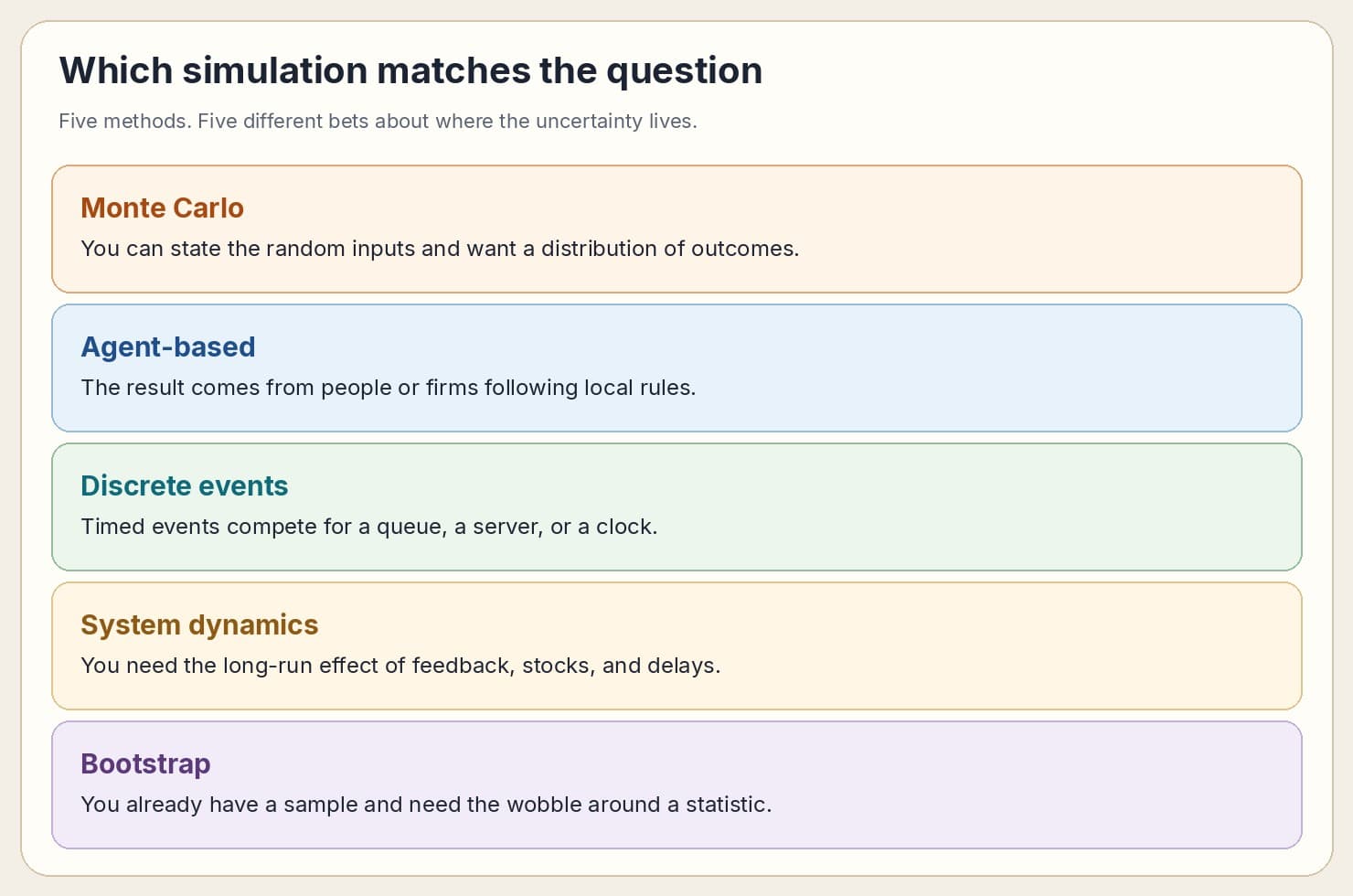
Choosing among them is a question about the uncertainty, not a ranking. If you can specify the random inputs and you want a distribution of outcomes, use Monte Carlo. If the behavior comes from different actors following local rules, use agents. If the system is timed events competing for resources, use discrete events. If you need the long-run effect of feedback, use system dynamics. If you already hold a sample and you need the uncertainty around a statistic, bootstrap it. Serious studies stack these. An agent or queue model can take uncertain parameters from a Monte Carlo loop, and the statistic at the end can be checked with a bootstrap.

Whatever you generate, write down what the artificial rows are allowed to claim. Simulated data can stress a pipeline, compare algorithms, and expose a bottleneck. It cannot replace a holdout set drawn from the process you will actually score later. Label the rows as simulated, keep the seed and the assumptions beside the result, and do not let a smooth distribution impersonate a population.

Used that way, simulation is a practical tool in a data-driven workflow: a way to test ideas and train models when the real extract is expensive, private, or not here yet. The five methods are different instruments for that job. As this work spreads, the scarce skill is not producing more random numbers. It is knowing which generator matches the question.

Sources. Cagle, K. (2023, March 13). 4 types of simulation models used in data analytics. TechTarget. https://www.techtarget.com/searchbusinessanalytics/tip/Types-of-simulation-models-used-in-data-analytics. MOSTLY AI. (2023, June 7). Data simulation: unlocking innovation and empowering organizations. https://mostly.ai/blog/data-simulation